Chapter 3 Fixed Income Features Calculations
In this chapter, the construction of spot rates, zero coupon bond prices, excess returns, and yield factors are discussed. These features are used in hedging strategies and for general exploration of the data in Chapters 4-5, so only the implementation is discussed here.
3.1 Spot Rates
Spot rates series can be constructed from the 6 parameters in the cleaned Federal Reserve data set. The following formula is used to construct the spot rates. It is integrated form of the Svensson extension of the Nelson and Siegal approach to calculating instantaneous forward rates. Svensson added a second hump term to the model that Nelson and Siegal created. Integrating the instantaneous forward rates gives us the spot rates.
\[ \begin{aligned} y_t(n) &= \beta_{0,t} \\ &+ \beta_{1,t} \frac{1 - \exp(- \frac{n}{\tau_{1,t}})}{\frac{n}{\tau_{1,t}}} \\ &+ \beta_{2,t} [\frac{1 - \exp(- \frac{n}{\tau_{1,t}})}{\frac{n}{\tau_{1,t}}} - \exp(-\frac{n}{\tau_{1,t}})] \\ &+ \beta_{3,t} [\frac{1 - \exp(- \frac{n}{\tau_{2,t}})}{\frac{n}{\tau_{2,t}}} - \exp(-\frac{n}{\tau_{2,t}})] \end{aligned} \]
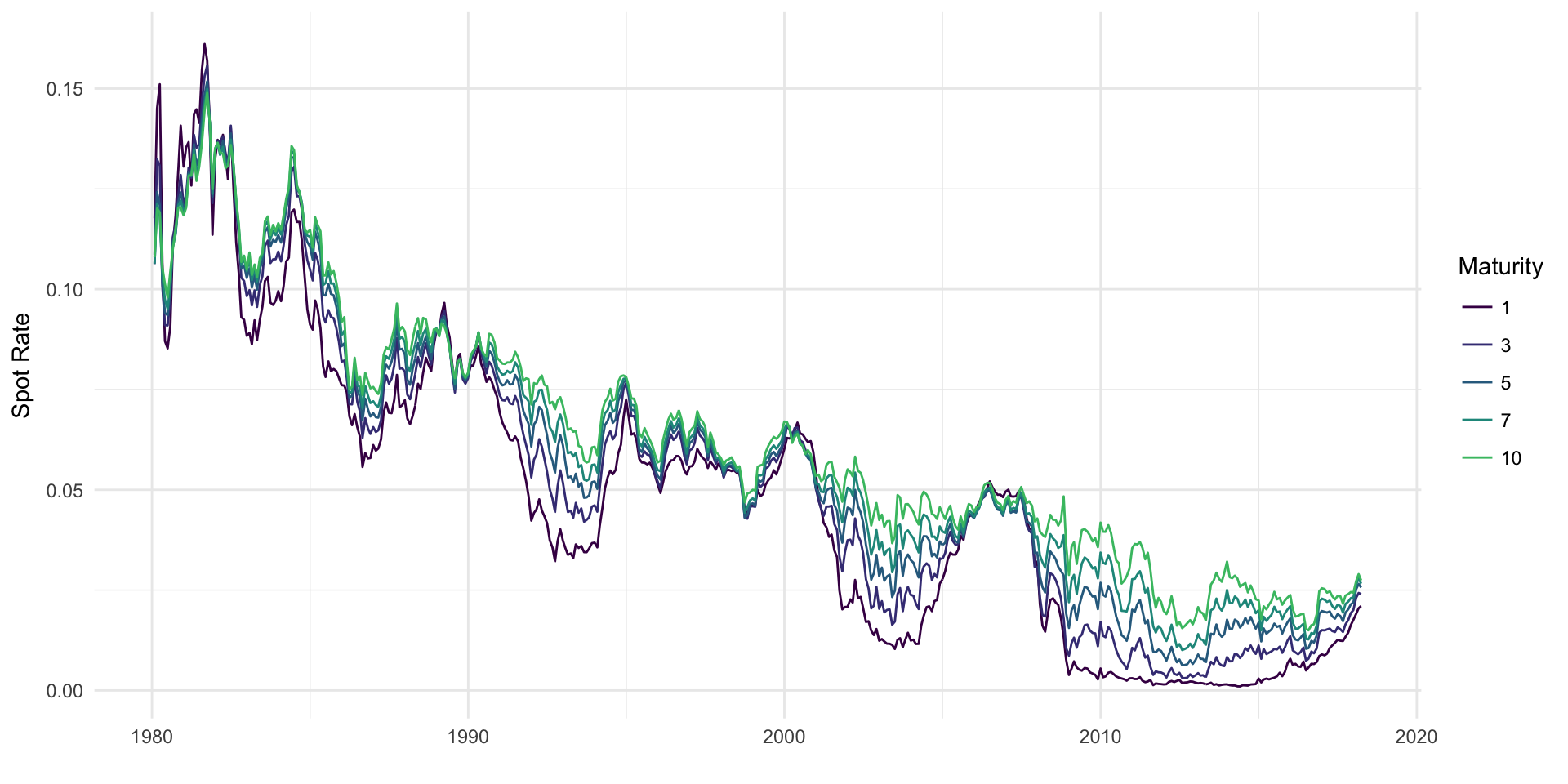
Spot rates are examined in detail in Chapter 4, but Figure 3.1 provides a quick look at the major ones. As expected, longer maturity spot rates are consistently higher than short term spot rates. The 1980’s were a time of incredibly high interest rates, and in recent years rates have been incredibly low.

Figure 3.1: Spot rates at various maturities from 1980 onward.
3.2 Zero Coupon Bond Prices
N-year zero coupon bond prices can be calculated easily from their corresponding spot rates. The following formula is used to represent the relationship between the two series.
\[ P_t(n) = \exp(-y_t(n) \times n) \]
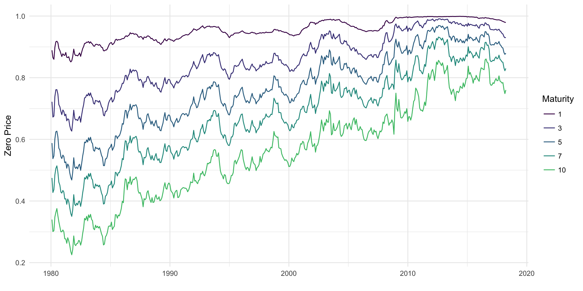
Zero prices, by design, exhibit an inverse relationship to spot rates. The impact of the high interest rates in the 1980’s can be seen clearly in Figure 3.2, with a large price spread between the short and long term maturity zeroes.

Figure 3.2: Zero prices at various maturities from 1980 onward.
3.3 One Month Returns
The time \(t+\Delta\) return on an n-year bond is defined as:
\[ RET_{t+\Delta}(n) = \frac{P_{t+\Delta}(n - \Delta)}{P_t(n)} - 1 \]
Using the zero coupon bond prices from Section 3.2, it is straightforward to calculate returns. Care must be taken to align the price from next month’s \(n-\Delta\) maturity bond with today’s \(n\) maturity bond, but otherwise the procedure is simple.
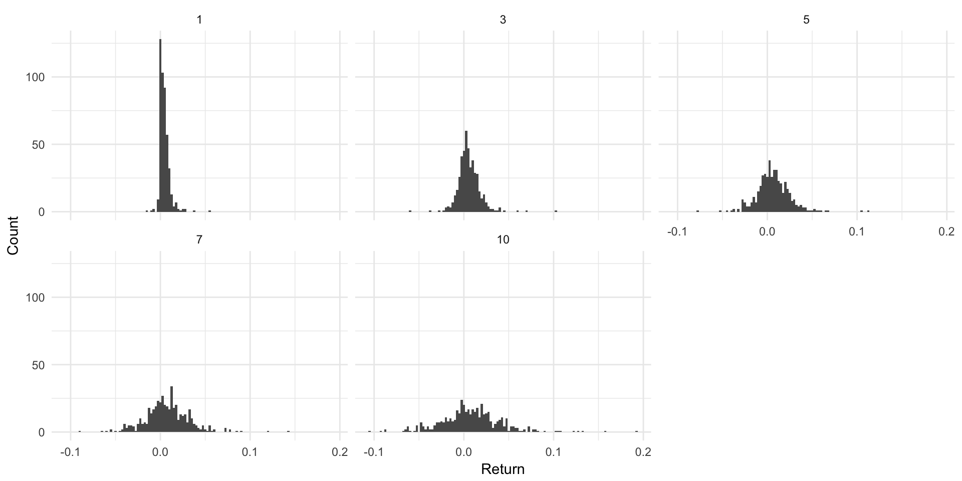
The distribution of 1-month (\(\Delta = 1/12\)) returns is shown in Figure 3.3. As seen in both the figure and Table 3.1, higher maturity zeros have both larger average returns and more variance. In general, this is unsurprising, and the drop in standard deviation is roughly linear as the maturity decreases.

Figure 3.3: Return distributions for various maturities.
| Maturity | Average Return | Standard Deviation |
|---|---|---|
| 1 | 0.0044510 | 0.0056046 |
| 3 | 0.0055643 | 0.0125839 |
| 5 | 0.0064662 | 0.0188464 |
| 7 | 0.0072532 | 0.0250410 |
| 10 | 0.0083056 | 0.0343082 |
3.4 Excess Returns
Excess returns are calculated over the 1 month treasury, specifically:
\[ ER_{t+\Delta}(n) = RET_{t+\Delta}(n) - RET_{t+\Delta}(\Delta) \]
with \(\Delta = 1 / 12\). Excess returns are only calculated for \(n = 1, 3, 5, 7, \text{and } 10\) year zeros.
The implementation of this is straightforward since returns for all maturities have already been calculated. Excess returns show a similar distribution as returns, just shifted downwards by the 1-month treasury return.
3.5 Yield Curve Factors
Finally, the yield curve factors, level, slope, and curvature are calculated as:
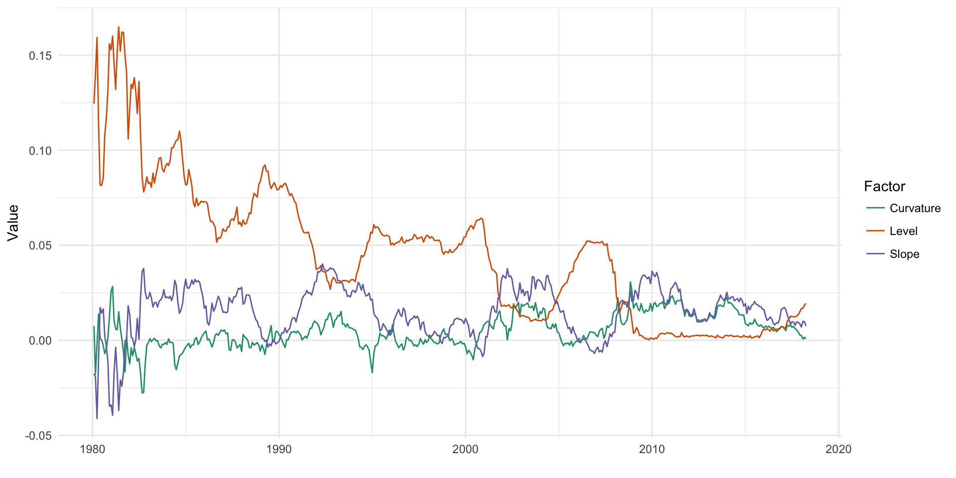
\[ \begin{aligned} \text{Level} &= y_t(1/4) \\ \text{Slope} &= y_t(8) - y_t(1/4) \\ \text{Curvature} &= [ y_t(8) - y_t(2) ] - [ y_t(2) - y_t(1/4) ] \end{aligned} \] As seen in Figure 3.4, the raw values of the yield curve factors do not offer much insight on their own, but they will be useful later in decomposing the spot rate and in multiplicative regression hedging.

Figure 3.4: Yield curve factors over time.