Chapter 6 Question 3
Question:
Perform the “out-of-sample” hedging exercises where \(n_h = 3\). Split the sample into two halves, such that \(T_0 = 2T\). Begin with the \(T\)-th month, calculate \(w_T(1)\), \(w_T(5)\), and \(w_T(10)\) for each hedging strategy, and save \(\epsilon_{T+\Delta}(n_h)\). Move forward and repeat the process each month, and calculate the root mean squared hedging error (RMSHE) for each strategy:
\[ RMSHE = [\frac{1}{T} \sum{\epsilon_{t+\Delta}(n_h)}]^{0.5} \]
Report your results and evaluate the performance of the hedging strategies.
Implementation details:
This chapter is broken into:
- 3 sections devoted to creating the modeling functions
- 1 section for creating a hedging error calculation function
- 1 section for creating an “interface” to the models and error calculations
- 1 section for running the models through the interface
- 1 section for reviewing model performance
The data for the \(y_t(1)\), \(y_t(3)\), \(y_t(5)\), \(y_t(7)\), and \(y_t(10)\) spot rates is required to calculate the durations for the zero coupon bonds used in the hedging exercises. Also required are the yield curve factors and excess returns. These have all been calculated in Section 3, and the results from there are used.
The models developed below will be structured in a way so that they can all be
fed with data from the same data set. To accomplish the rolling out-of-sample
technique, the rsample package was used. Specifically, the rolling_origin() function
was utilized which allows easy splitting of data into rolling sets of 230 months,
which is the T value corresponding to half of the data.
6.1 Modified / Macaulay Duration
The first two strategies involve creating duration matched barbells using 1-year
and 10-year zero coupon bonds to match the duration of a 3-year or 7-year bullet.
Since the strategies are essentially the same, one modeling function is used for both, model_duration(),
with an argument to select whether to use modified or macaulay duration. The duration
is calculated using the duration() function in the ratekit package
and the barbell weights are calculated with the barbell_weights() function.
The function is created in such a way that it accepts a single split from the
total data frame, and calculates the weights for just that one split.
The weight for a 5-year zero is included to be consistent with the other models,
but is set to 0.
6.2 Simple Regression Based Hedging
The regression based hedging method involves the regression:
\[ ER_t(n_h) = w_t(1) ER_t(1) + w_t(5) ER_t(5) + w_t(10) ER_t(10) + u_t(n_h) \]
The R function lm() is used to run the regression, and the weights are
extracted and returned in the same format as the duration models. This is all
wrapped into a modeling function, model_regression().
6.3 Multiplicative Regression Hedging
The multiplicative regression follows the model:
\[ ER_t(n_h) = \theta_t(1; X_{t-\Delta}) ER_t(1) + \theta_t(5; X_{t-\Delta}) ER_t(5) + \theta_t(10; X_{t-\Delta}) ER_t(10) + u_t(n_h) \] where \(\theta_t(n; X_{t-\Delta})\) depends on the yield curve factors as:
\[ \theta_t(n; X_{t-\Delta}) = a_t(n) + b_t(n) \text{Level}_{t-\Delta} + c_t(n) \text{Slope}_{t-\Delta} + d_t(n) \text{Curvature}_{t-\Delta} \]
Once the models are fit, the weights at time \(t\) can be calculated as \(\theta_t\) values using the yield curve factors at \(t\):
\[ w_t(1) = \theta_t(1; X_t) \\ w_t(5) = \theta_t(5; X_t) \\ w_t(10) = \theta_t(10; X_t) \]
The entire procedure is wrapped into model_multiplicative_regression(), which,
consistent with the other model_*() functions developed so far, accepts a single
rolling split, along with the type of bullet (3 or 7-year), and returns the weights.
6.4 Error Calculation
Hedging error for the weights set at time \(t\) are calculated at time \(t+\Delta\) as:
\[ \epsilon_{t+\Delta} = w_t(1) ER_{t+\Delta}(1) + w_t(5) ER_{t+\Delta}(5) + w_t(10) ER_{t+\Delta}(10) \] These weights are then aggregated using RMSHE to determine overall model performance.
6.5 Model Selection Interface
A practical way to call all of the above models would be through an interface function that take as parameters: the data, the model to run, and the bullet to hedge against. Such a function was developed, and returns a data frame of the model type, the bullet used, the date of the error calculation, the weights, and the hedging errors.
6.6 Model Application
Finally, a data frame of function calls and parameter sets is created to easily iterate over all of the models. This data frame has a very compact form:
invokable## # A tibble: 8 x 2
## f params
## <chr> <list>
## 1 apply_model <list [3]>
## 2 apply_model <list [3]>
## 3 apply_model <list [3]>
## 4 apply_model <list [3]>
## 5 apply_model <list [3]>
## 6 apply_model <list [3]>
## 7 apply_model <list [3]>
## 8 apply_model <list [3]>The first column contains the function interface, apply_model(). Each element of the params column contains the data to be used in the model,
the model type, and the bullet to hedge against.
invokable$params[[1]]## $.data
## # Rolling origin forecast resampling
## # A tibble: 229 x 2
## splits id
## <list> <chr>
## 1 <S3: rsplit> Slice001
## 2 <S3: rsplit> Slice002
## 3 <S3: rsplit> Slice003
## 4 <S3: rsplit> Slice004
## 5 <S3: rsplit> Slice005
## # ... with 224 more rows
##
## $model
## [1] "modified_duration"
##
## $bullet
## [1] "3"6.7 Model Results
Table 6.1 displays the RMSHE results from each model. The regression methods significantly outperformed the duration based models, with much lower RMSHE. Among the duration models, Macaulay duration did marginally better, but the statistical significance is likely negligible. Among the regression models, the multiplicative regression did slightly better than the simple regression with the 3-year bullet and slightly worse with the 7-year bullet. The results are so close, however, that I am inclined to conclude that the simpler regression model is the best and most parsimonious model of the four. There is little to indicate that longer maturity bullets are harder to hedge than shorter maturity bullets. In fact, with the regression models, the opposite seems to be true.
| Model | Bullet | RMSHE |
|---|---|---|
| Macaulay | 3 | 0.0038994 |
| Macaulay | 7 | 0.0039961 |
| Modified | 3 | 0.0039390 |
| Modified | 7 | 0.0040058 |
| Multipl. Regression | 3 | 0.0008060 |
| Multipl. Regression | 7 | 0.0007763 |
| Regression | 3 | 0.0008178 |
| Regression | 7 | 0.0007663 |
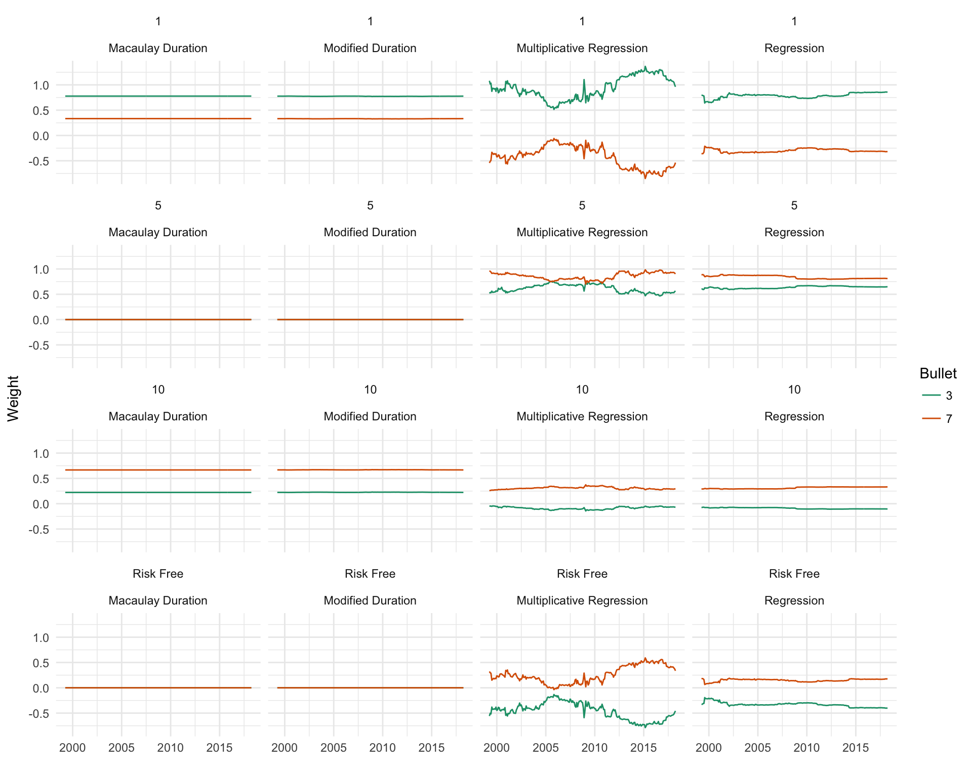
Because a rolling model was fit, a similar analysis can be performed as Section 5.6 where the stability of the coefficients over time was analyzed. In this case, the assignment of hedging weights by the models over time can be analyzed rather than just the coefficients. Some interesting insights can be gathered from Figure 6.1. Keeping in mind that duration models are only allowed to assign weight to a 1 year and 10 year zero, it is interesting to see how stagnant the weighting is between the 1 year and 10 year. The fact that the model essentially does not have the flexibility to vary the weights much over time likely contributes to its poor performance. The duration model also never shorts, which likely helps the regression models. The weightings in the duration models do make sense, with more than 50% being assigned to the 1-year bond to hedge the 3-year bullet, and more than 50% being assigned to the 10-year the hedge the 7-year bullet. In the regression models, there is an implicit risk free instrument that weight can be assigned to, so a 4th row in the figure is included to incorporate that. The simple regression model only shifts weights around in periods of high stress, 2001 and the jump around 2008 being two examples, but even so, the weightings are surprisingly stable over time. This is especially apparent when contrasted with the multiplicative regression. Weights are highly varied over time, but the performance gain for this is limited as seen in the RMSHE results, questioning the need for the complex model.

Figure 6.1: Hedging weight assignment over time
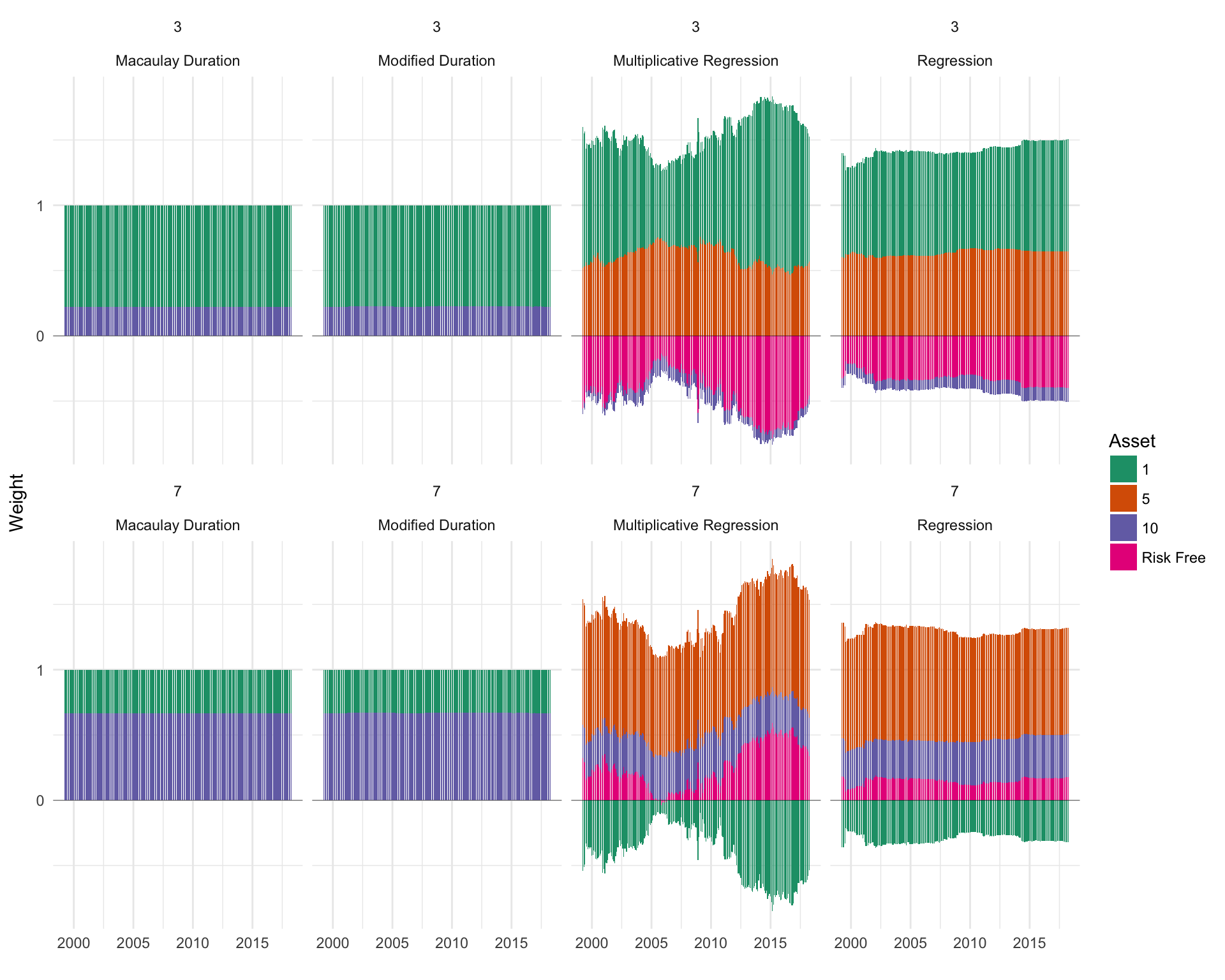
Another way to view the weights over time is by stacking them. This is done in Figure 6.2 and provides another unique view into the change in the total weight distribution over time. This view confirms the stagnant weights in the duration models, but also offers some other new insights. In the regression models, hedging the 3-year bullet requires shorting the 10-year and the risk free, while hedging the 7-year bullet only required hedging the 1-year bond. This view also further demonstrates the wild swings in the multiplicative regression, for questionable performance gains.

Figure 6.2: Stacked weight assignment over time